Simulate DC IR drop (experimental)

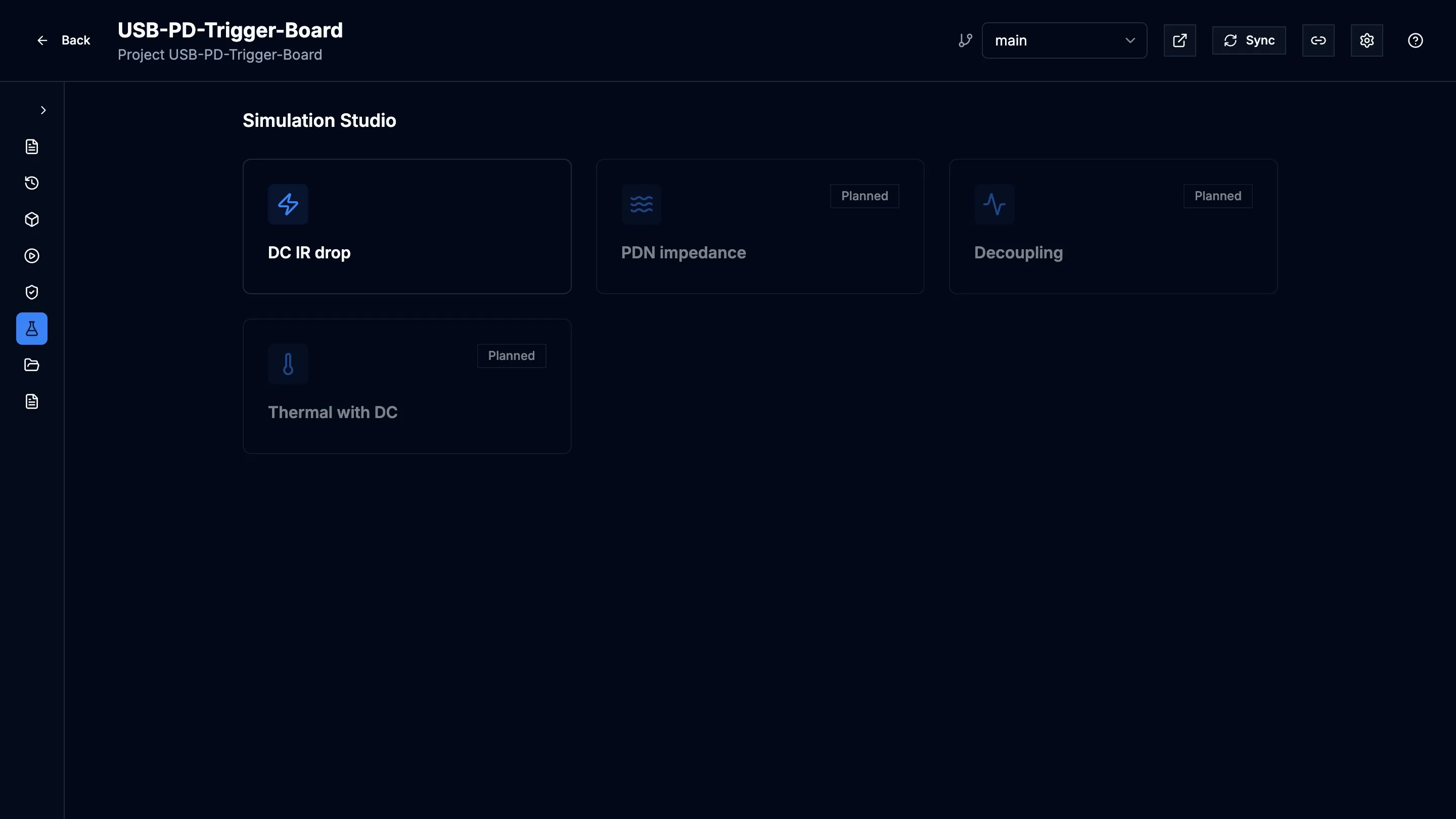
Simulation Studio runs board-level simulations on a revision of your project. Its first analysis is DC IR Drop: you describe the board’s power tree (sources, converters, rails and loads), and Prism solves the voltage drop and current density in the copper and draws the result on the board.

Simulation Studio: DC IR Drop available, with PDN impedance, Decoupling and Thermal with DC marked Planned

Who can do what

Viewers can open setups and results. Designers and admins can create and edit setups and start runs.

Create a setup

A setup holds one power tree, its loads and its solver settings. You can keep several setups per project, for example one per operating mode.

Open the project and choose Simulation Studio.
Select DC IR Drop. Analyses marked Planned are not available yet.
Select New setup.
Enter a Setup name.
In Start from, choose Inferred power tree to begin with the power tree Prism reads from the netlist, or Blank canvas to build it yourself.
Select Create.

The setup uses the project’s current revision. That revision’s design data must be ready before you can run it.

Build the power tree

The Setup tab shows the power tree as a canvas.

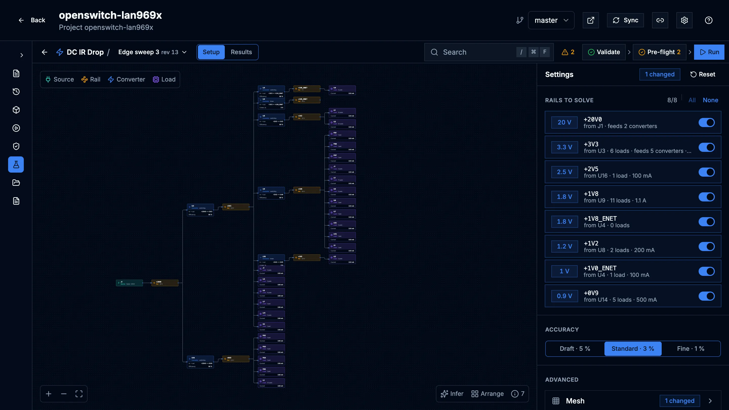
The Setup tab of an OpenSwitch LAN969x setup: the power tree canvas from the 20 V input through its converters to the loads, and the Settings panel listing the rails to solve and the accuracy

Add elements adds a Source, Converter, Rail or Load. Pick the part or net it belongs to from the board.
Select an element to edit it in the inspector: for example a source’s Voltage, a converter’s Input rail, Output rail and type (Switching (efficiency) or Linear (passes its current)), or a load’s Current.
Infer fills an empty canvas from the netlist (Shift+I). On a canvas that already has elements, choose Add missing to keep your elements and values, or Replace tree, which discards the currents and efficiencies you set.
Inference notes lists what the inference could not work out on its own.
Arrange lays the tree out again (A).
Settings holds the solver settings, such as Accuracy (Draft · 5 %, Standard · 3 % or Fine · 1 %) and the rails to solve. Settings you change from the default are marked.

You can also search the board from the header and jump to a part or net in the tree.

Prism saves each edit as a new revision of the setup. If someone else saved the setup since you opened it, your edit is refused instead of overwriting theirs; reload and try again.

Check and run

The header has three steps, left to right:

Validate checks the setup for missing or inconsistent values.
Pre-flight checks that the solver can run it against this board.
Run freezes this revision of the setup and queues the simulation.

Validate and Pre-flight run by themselves after each save, and you can run them again from their buttons. Run is available once Pre-flight passes. Any problems from the last check are listed in the issues button; select one to jump to the element it concerns.

If the revision’s design data is still being prepared, the run fails with a message asking you to run again when it is ready.

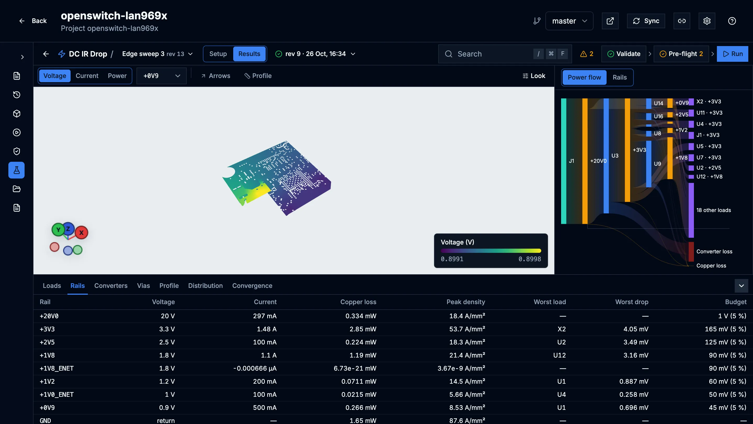
Read the results

Open the Results tab. It shows a spinner while a run is queued or running. With more than one run, pick the one to show from the run list.

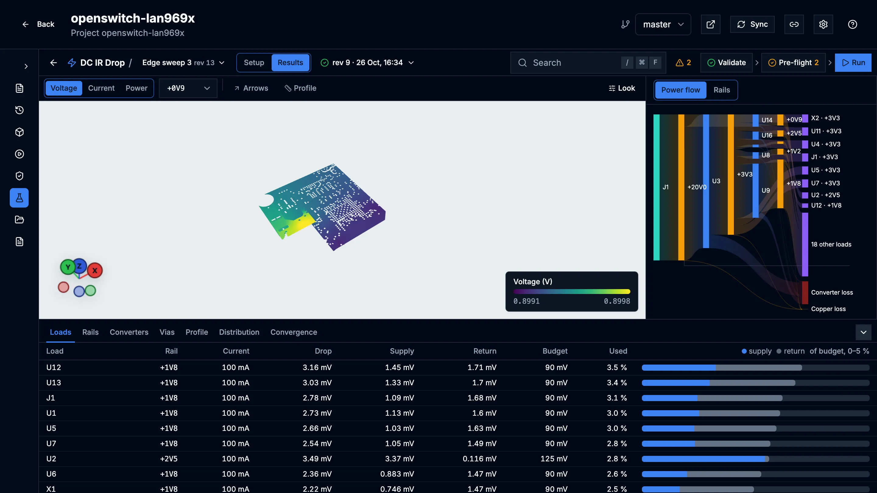
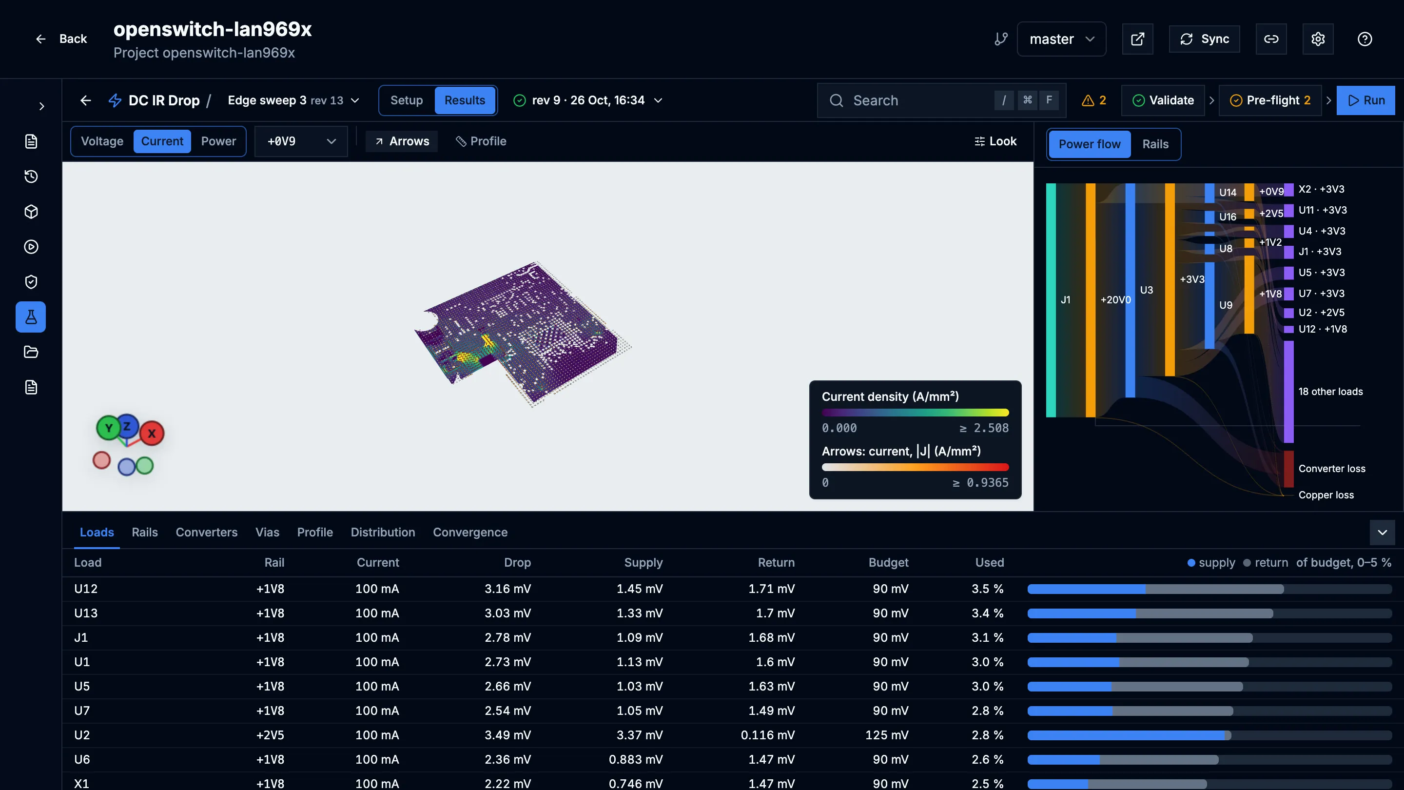
Results for the same board: the copper coloured by voltage on the +0V9 rail with its scale, a power-flow chart from the input through each rail to the loads and losses, and the Loads table with each load’s drop, supply and return share against its budget

The board view colours the copper by voltage drop, current density or power density, with optional current arrows. Colours and arrows adjusts how they look.
The side panel summarises each rail and load, with a Chart of the results.
The analysis drawer has the power budget (supply, converter loss, copper loss), via currents, convergence, and a Profile: draw a line on the copper to plot the field along it.
Back to setup returns to the setup that produced the run.

Current density on the copper with current arrows, and the arrow scale

The Rails tab: each rail’s voltage, current, copper loss, peak density, worst load and worst drop against its budget

Script the studio from the browser

While Simulation Studio is open, the browser console has a window.prismSimStudio object that performs the same operations as the interface, as the signed-in user. For example:

const s = await prismSimStudio.newSetup("Max load", { seed: "inferred" });
await prismSimStudio.updateElement(s.setup_id, "load:u1-0v9", { values: { current_a: 3 } });
await prismSimStudio.validate(s.setup_id);
await prismSimStudio.preflight(s.setup_id);
await prismSimStudio.submit(s.setup_id);

Elements are named kind:id, such as rail:3v3, converter:u3-3v3, load:u1-0v9 or source:j1-20v0. prismSimStudio.tree(setupId) shows the names in a setup.

Limits

DC IR drop is the only analysis available.
Prism keeps a limited number of runs per setup and deletes older ones automatically. Ask your administrator if you need runs kept longer.